
An Analytical Laboratory Chiller Is Sized by Peaks, Not Averages
Coal quality analyzers and Kjeldahl digestion systems look like different instruments and produce the same cooling problem: a burst of heat during a determination, then almost nothing until the next sample.
That pattern breaks the usual sizing approach. Average the load over a shift and the number looks trivial — a couple of hundred watts, well inside anything on the market. Size on that average and the temperature climbs during every determination, which is precisely when the measurement is being taken.
This is a guide to sizing an analytical laboratory chiller for intermittent duty: how to find the peak, what thermal mass does and does not buy you, and why stability matters more here than in almost any other benchtop application.
Why These Instruments Share a Profile
Both instrument families run a cycle: heat the sample hard, then cool the condensate or the jacket, then idle while results are read and the next sample is prepared.
Coal quality analyzers — proximate analysis, calorific value determination, sulfur analysis — heat samples to high temperatures and need the surrounding equipment held stable. The heat arriving at the cooling loop is concentrated in the determination window.
Kjeldahl systems — digestion followed by distillation — produce a substantial condenser duty during the distillation step and very little between runs.
Two consequences follow from that shared shape, and they pull in opposite directions. The average load is low, which tempts you toward a small machine. The peak load is not, and it arrives exactly when accuracy matters.
Finding the Peak
Sizing an analytical laboratory chiller starts with a number most people never measure. Three approaches, in descending order of reliability.
Measure it. If the instrument is already running, put a thermometer on the supply and return of the cooling loop and record through a determination at a known flow. Q = flow (L/min) × 69.7 × ΔT (°C). The highest value during the cycle is your peak.
Calculate from the process. For a Kjeldahl distillation, the condenser duty follows the boil-up rate: kilograms per hour times latent heat divided by 3.6 gives watts. Water at 1 L/h is roughly 628 W, which is why aqueous distillation is a heavier duty than solvent work.
Bound it electrically. Whatever the instrument draws from the wall is an upper limit on what it can dissipate. Coarse, but it catches order-of-magnitude errors.
Typical peaks for benchtop instruments in these families land in the 200–600 W region, with the average across a working day considerably lower.
How precisely a benchtop machine can hold a setpoint, and what determines it, is covered in lab chiller temperature control.
What Thermal Mass Buys — and What It Does Not
The reservoir is more useful here than in most applications, and it is worth being precise about why.
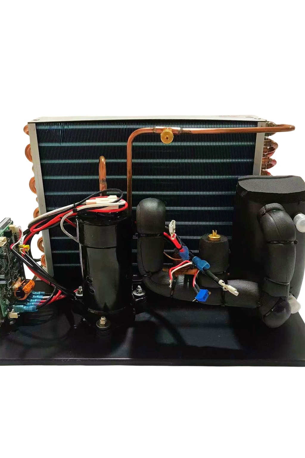
During a determination, the instrument dumps heat faster than the refrigeration circuit alone can remove it. The fluid volume absorbs the difference, rising in temperature rather than letting the instrument overheat. Between determinations, the refrigeration circuit removes what the reservoir absorbed and the temperature returns.
So thermal mass converts a sharp thermal spike into a gentle rise and recovery. Whether that is enough depends on three things:
- How large the peak is relative to the machine’s capacity. A peak twice the capacity for two minutes is very different from a peak twice the capacity for an hour.
- How long the determination lasts. The longer the burst, the more the reservoir has to absorb, and the further the temperature drifts.
- How much time there is before the next sample. Recovery needs the idle period. A busy day with back-to-back determinations removes the recovery time the buffering strategy depends on.
That last point is the one that catches laboratories out. A machine sized adequately for occasional use becomes marginal when throughput rises, because the assumption it relied on was idle time rather than capacity.
The Rule That Follows
Two sizing approaches, and which one applies depends on your tolerance.
If the process tolerates a temperature rise during the determination — the measurement is not sensitive to a couple of degrees at the cooling loop — size somewhere between the average and the peak, and let the reservoir absorb the difference. Confirm the recovery time is shorter than the interval between samples.
If the process does not tolerate it — where the cooling temperature affects the result — size against the full peak. The reservoir then becomes margin rather than the mechanism you rely on.
For calorimetric work in particular, the second approach is the honest one: a calorimeter measures heat, so drift on the cooling side becomes measurement error rather than an inconvenience.
For choosing across the wider laboratory range, see choosing the right laboratory chiller and the recirculating chiller selection guide.
Stability Is the Specification Here
In most benchtop applications capacity decides the machine. In analytical instrumentation it frequently does not.
The reason is reproducibility. If the cooling temperature differs between the morning run and the afternoon run, a systematic difference appears in the results that has nothing to do with the samples. Determinations that are compared against each other — batch to batch, laboratory to laboratory, against a reference — inherit whatever the cooling loop was doing.
Two specifications matter:
How the machine controls. An on/off controller switches around the setpoint and produces a sawtooth several degrees wide. A modulating controller varies compressor speed to match the load and holds much closer to a line. Where a figure of ±0.1 °C is quoted, it describes modulating behavior.
Where the sensor sits. Stability quoted at the reservoir is not the same as stability at the instrument, particularly on a long or uninsulated tubing run.
Sizing Table
Three instrument families against the figures that decide the analytical laboratory chiller.
| Coal analyzer | Kjeldahl system | Calorimeter | |
|---|---|---|---|
| Load pattern | Burst per determination | Burst during distillation | Low but continuous |
| Typical peak | 200–600 W | 300–600 W | 200–500 W |
| Typical setpoint | 10–20 °C | 10–20 °C | 15–25 °C |
| Binding constraint | Peak and recovery time | Boil-up rate | Stability, not capacity |
| Reservoir value | High | Moderate | Moderate |
| Tolerance to drift | Depends on method | Usually some | Very low |
Read the bottom two rows together. Where drift tolerance is low, the reservoir stops being a substitute for capacity and becomes only a safety margin.
Sharing One Machine Between Instruments
Whether one analytical laboratory chiller can serve a whole bench is a common question, and the arithmetic is not simply additive. A laboratory with several of these instruments naturally asks whether one chiller can serve them all.
Peaks may not coincide — but plan as if they do. If two instruments can run simultaneously, the design case is both peaks together, not an averaged figure.
Setpoints do not add. One loop runs at one temperature, and the coldest requirement wins. If one instrument wants 10 °C and another 20 °C, both get 10 °C.
Flow adds, and resistance compounds. Instruments in series see the same flow but their pressure drops add. In parallel, the split follows resistance rather than intention, and the less restrictive branch takes more.
One instrument disturbs another. This is the decisive one. A burst from an analyzer moves the loop temperature that a calorimeter was relying on. Where one instrument is stability-critical and another produces transients, separate loops are the honest answer even when a single machine could carry the total watts.
Placement matters in a room where measurements are being taken — vibration and acoustic isolation covers where to put the machine.
Water Quality Matters More Than the Duty Suggests
Intermittent operation has one consequence that steady-duty applications avoid, and it affects the fluid rather than the machine.
A loop that runs continuously stays at a stable temperature and keeps moving. A loop serving an analytical laboratory chiller spends much of its life warm and still, cycling through temperature every time a determination runs. Two things follow.
Thermal cycling accelerates scale. If the loop was filled with tap water, dissolved minerals precipitate onto the hottest surface each time the system works, and the cycling gives more opportunities than continuous running at a steady temperature would. The deposit insulates the heat exchanger and is effectively permanent.
Warm and still is a good habitat. Biological growth needs warmth and time, and an intermittent loop provides both. The result is biofilm on internal surfaces and loose material at the filter, which presents as reduced flow rather than reduced capacity.
Neither is difficult to prevent. Fill with distilled or deionized water — not tap, not bottled drinking water, both of which carry dissolved minerals. Keep light off the loop by using opaque tubing and a covered reservoir. And check the fluid on condition rather than on a calendar: discoloration, odor, sediment, or rising conductivity are the signals, and any of them appearing early suggests the fill was wrong rather than that the interval was too long.
The failure this prevents is worth naming, because it looks like something else. A scaled heat exchanger reduces capacity gradually over months, which reads as a machine that is no longer big enough — and replacing it with a larger one repeats the same process on new hardware.
Where a Countertop Unit Fits
Peaks of a few hundred watts, setpoints in the 10–25 °C region, reproducibility mattering more than raw capacity, on instruments that sit on a bench in a room with people working — that is the profile these machines are built for.
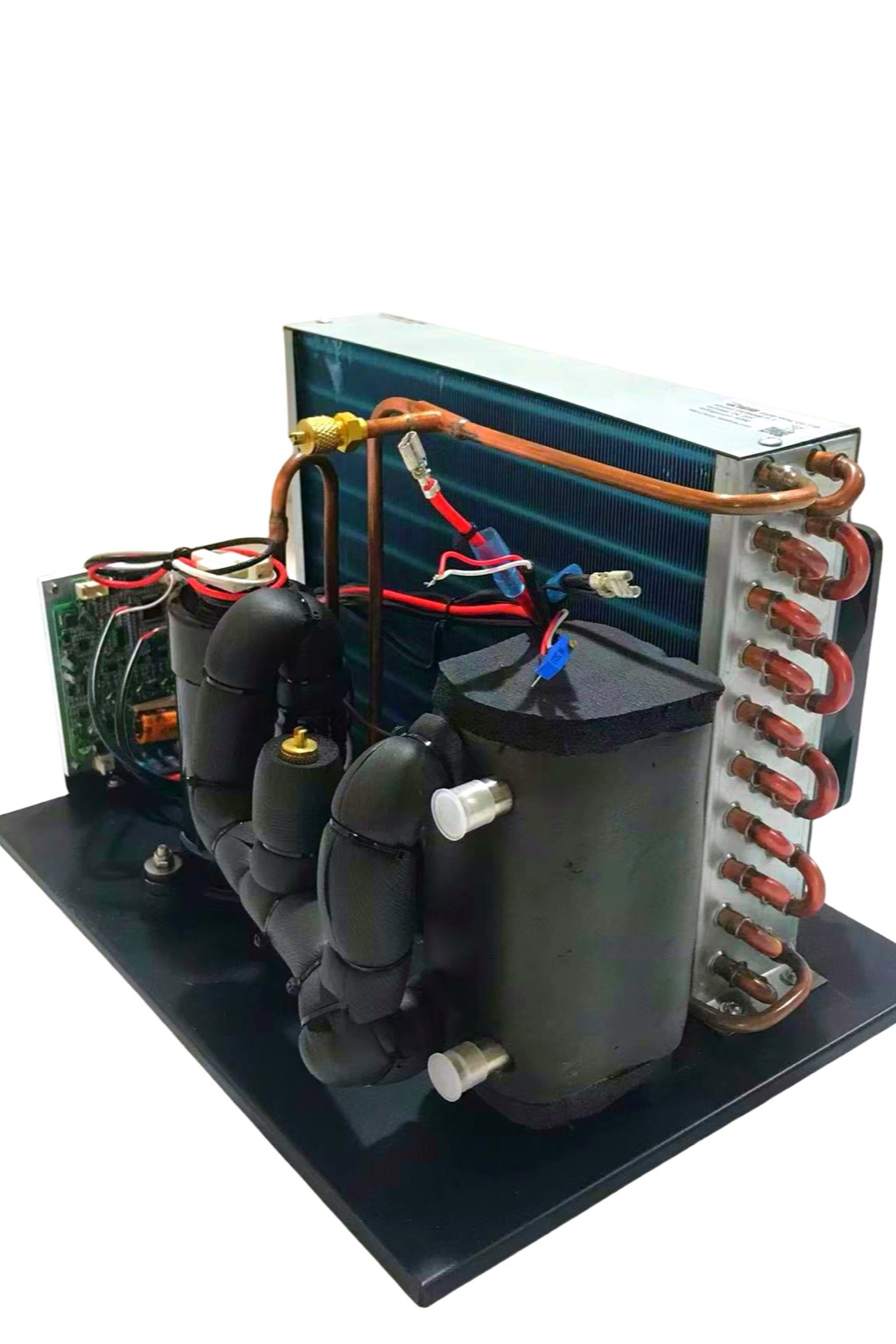
The setpoints in the table sit between 10 and 25 °C, and that span crosses a product boundary. From +10 to +20 °C the DV-series compact liquid chiller covers the duty: 100–550 W across a −20 to +20 °C range, on 12 V, 24 V or 48 V DC with R134a or R290, in plate, coaxial and coil formats — a plate unit such as the DV1910E-P measures around 330 × 200 × 138 mm. Confirm the configuration against your load. From +20 to +25 °C you are past that line’s published ceiling: that band needs engineering confirmation, or a complete recirculating platform explicitly rated for the warm range. One catalog note worth making explicitly: the MiniCool range lists coal analyzers and Kjeldahl apparatus among its intended instruments, but its published span is 0 °C to −40 °C, so for these warm loops the DV line is the one whose range covers the duty. And where a measured peak exceeds 550 W at a warm setpoint, neither line’s published figures cover it — that case is a question for engineering rather than a catalog choice.
Two things to establish before choosing. The published capacities do not state their test temperature, so ask for the figure at your setpoint. And reservoir volume is not published, which matters here because the buffering strategy depends on it.
The compact liquid chiller page lists the formats. Contact the Arctic-Tek engineering team with your measured peak, the determination duration, the interval between samples, and how much drift your method tolerates — those four decide whether you are sizing against the peak or against the average.
Frequently Asked Questions
Should I size for the peak or the average load?
Against the peak if the measurement is sensitive to cooling temperature. Between the two if it is not, provided the recovery time between determinations is shorter than the interval between samples.
Does a bigger reservoir let me use a smaller machine?
Partly, and only for short bursts with adequate idle time afterward. Against a sustained load or back-to-back determinations, thermal mass delays the problem rather than solving it.
Why does stability matter more than capacity for analytical work?
Because a difference in cooling temperature between runs becomes a systematic difference in results. Reproducibility depends on the loop holding the same value every time, not on how many watts it can remove.
Can one chiller serve several instruments?
If the combined peak fits, the pump delivers the total flow, and the shared setpoint suits all of them. But a transient from one instrument disturbs the others, so stability-critical work usually wants its own loop.
What happens if throughput increases later?
A machine relying on idle time for recovery becomes marginal when determinations run back to back. If throughput is likely to rise, size against the peak rather than the average.
Summary
An analytical laboratory chiller for coal analyzers, Kjeldahl systems, and calorimeters is sized by peak rather than average, because the heat arrives in bursts that coincide with the measurement. Find the peak by measuring across a determination or calculating from the boil-up rate; typical figures land between 200 and 600 W. Thermal mass converts a spike into a gentle rise, but only where there is idle time to recover in — which is the assumption that fails first when throughput increases. Above all, treat stability as a separate specification from capacity: for instruments whose results are compared against each other, a loop that drifts between runs introduces a systematic error that no amount of cooling capacity corrects.